The Art Of Packing Data

The packing of data is good practice for many reasons, including disk space and efficient RAM or cache access. If we know the meaning of data we can often narrow down the range and precision, making informed decisions as to the amount of bytes we need. I was inspired once by this article and here’s my take on the topic. We’ll explore common ways of packing certain kinds of data common in videogames, their possible implementation and rationale; worthy of note is that this is not an article about compression. I’ll be using HLSL syntax but this will look very familiar to C++ and can be ported easily to any other language.

Normalized Data

This is the simplest type of data to pack so we’ll start here. Normalized data ranges from 0 to 1. You can easily normalize data by shifting and dividing by its maximum value. This mostly applies to colors or bounded values (think a shadow or transparency term) and sometimes normalized vectors, although there are better methods as we’ll see later. The D3D12 formats for this kind of data are the _UNORM class, such as R8G8B8A8_UNORM or R16G16_UNORM. The code examples below show how to encode a typical color with alpha into 8 and 16 bits, they are common cases but you can make as many variations as needed depending on the bitrate and the data you want to store.

Note how we add 0.5 to the result after multiplying by 255. This operation followed by casting is equivalent to rounding but avoids the round instruction since the add gets factored into the multiply-add. Some of these operations are so common that many closed platforms have intrinsics or special instructions to encode and decode bits. Recently, HLSL added some special packing instructions to Shader Model 6.6 so we can also write the RGBA8 packing as follows.

We’ll stop here for a minute to analyze the RDNA bytecode generated from these instructions. I have grouped them to make logical sense as the compiler is free to reorder these. These tests were performed on the Radeon Graphics Analyzer using the 1103 RDNA3 ASIC in offline mode. We need to be careful as older RGA versions produce worse than the baseline, whereas the latest one I used here shows an improvement. As always, measure and make sure! The command line I used, should you wish to replicate the results, is .\rga.exe -s dx12 -c gfx1103 –offline –cs example.hlsl –cs-entry CSMain –cs-model cs_6_6 –dxc-opt –isa example_hlsl_v1.txt

1 2 3 4 5 uint PackFloat4ToRGBA8Unorm(float4 value) {     uint4 uvalue = uint4(value * 255.0 + 0.5);     return (uvalue.a << 24) | (uvalue.b << 16) | (uvalue.g << 8) | uvalue.r; }

1 2 3 4 5 uint PackFloat4ToRGBA8Unorm(float4 value) {     uint4 uvalue = uint4(value * 255.0 + 0.5);     return pack_u8(uvalue); }

1 2 3 4 5 6 7 8 9 10 11 12 13 14 15 16 17 18 19 20 // MAD 255.0 + 0.5 (4 instructions) v_fma_f32     v4, s6, lit(0x437f0000), 0.5 v_fma_f32     v1, s4, lit(0x437f0000), 0.5 v_fma_f32     v3, s7, lit(0x437f0000), 0.5 v_fma_f32     v2, s5, lit(0x437f0000), 0.5 // Convert to integer (4 instructions) v_cvt_i32_f32  v4, v4 v_cvt_i32_f32  v1, v1 v_cvt_i32_f32  v3, v3 v_cvt_i32_f32  v2, v2 // Shift left (3 instructions) v_lshlrev_b32  v3, 24, v3 v_lshlrev_b32  v2, 8, v2 s_lshl_b32    s4, s4, 16 // OR them all together (3 instructions) v_or_b32      v1, s4, v1 v_or_b32      v1, v3, v1 v_or_b32      v2, v2, v1   Total: 14 instructions

1 2 3 4 5 6 7 8 9 10 11 12 13 14 15 16 // MAD 255.0 + 0.5 (4 instructions) v_fma_f32     v0, s4, lit(0x437f0000), 0.5 v_fma_f32     v1, s5, lit(0x437f0000), 0.5 v_fma_f32     v2, s6, lit(0x437f0000), 0.5 v_fma_f32     v3, s7, lit(0x437f0000), 0.5 // Convert to integer (4 instructions) v_cvt_i32_f32  v0, v0 v_cvt_i32_f32  v2, v2 v_cvt_i32_f32  v3, v3 v_cvt_i32_f32  v1, v1 // Permute and OR (3 instructions) v_perm_b32    v2, v2, v3, lit(0x00040c0c) v_perm_b32    v0, v0, v1, lit(0x0c0c0004) v_or_b32      v0, v2, v0   Total: 11 instructions

As you can see the compiler is able to improve our hand-written logic and squeeze a couple extra instructions for our packing using v_perm_b32, an instruction that swizzles values into a single one. We don’t have the high-level instructions to perform the same operations manually which is unfortunate. There are other normalized formats commonly used in videogames that don’t have the same bit width for all components, for example R5G6B5, R5G5B5A1 or R10G10B10A2 formats. We can see how to encode and decode one of them below.

Signed Normalized Data

Encoding positive normalized data works well with the method above. When the normalized data can be negative as well, unexpected things can happen if we’re not careful. For example, let’s try to encode a normal vector pointing upwards (0, 1, 0) using what we know so far.

Notice how zero cannot be represented exactly and now the decoded vector is tilted slightly sideways (always biased towards +xz in a positive y coordinate system). If you’re using something like this to encode normals for vertex data or in textures, you’ll see e.g. mirror reflections looking slightly tilted instead of properly aligned. We can see why visually:

0	1	…	126	127	128	129	…	254	255
-1.0	-0.992156	…	-0.011764	-0.003921	0.003921	0.011764	…	0.992156	1.0

Signed normalized data formats, such as the D3D12 formats in the _SNORM class, have a couple of special rules that help us fix the above problem. Reading the DirectX documentation in this regard, we’ll see this small snippet:

The minimum value means -1.0f (e.g. the 5-bit value 10000 maps to -1.0f). In addition, the second-minimum number maps to -1.0f (e.g. the 5-bit value 10001 maps to -1.0f). There are thus two integer representations for -1.0f. There is a single representation for 0.0f, and a single representation for 1.0f

The whole point of the above paragraph is to make sure we are able to accurately represent 0, even if we need to lose one of the values and repeat the value -1.

-128	-127	-126	…	-2	-1	0	1	2	…	126	127
-1.0	-1.0	-0.992125	…	-0.01574	-0.00787	0.0	0.00787	0.01574	…	0.992125	1.0

We now present the code to pack and unpack. Notice how we use round to make sure we add 0.5 for positive numbers and subtract 0.5 in the case of negative numbers. Worthy of note too is that we need to operate with ints instead of uints to get sign extension. Simply masking the bits and casting to int won’t preserve the sign bit, which is the reason we shift left and shift back right. It’s the same thing that happens in C++ (conceptually) when casting a char to int. Fortunately for us the compiler knows exactly what we want to do and removes the shifts using the bitfield extract instruction (v_bfe_i32) which we’ll see later.

An alternative version using the pack_s8 HLSL 6.6 intrinsic provides us with some gains too, code below using RGA as well.

1 2 3 4 5 uint PackFloat4ToRGBA8Snorm(float4 value) {     int4 ivalue = int4(round(value * 127.0)) & 0xff;     return (uint)((ivalue.a << 24) | (ivalue.b << 16) | (ivalue.g << 8) | ivalue.r); }

1 2 3 4 5 uint PackFloat4ToRGBA8Snorm(float4 value) {     int4 ivalue = int4(round(value * 127.0));     return (uint)pack_s8(ivalue); }

1 2 3 4 5 6 7 8 9 10 11 12 13 14 15 16 17 18 19 20 21 22 23 24 25 26 27 // MUL * 127.0 (4 instructions) v_mul_f32     v3, lit(0x42fe0000), v3 v_mul_f32     v2, lit(0x42fe0000), v2 v_mul_f32     v4, lit(0x42fe0000), v4 v_mul_f32     v1, lit(0x42fe0000), v1   // Round for fair distribution (4 instructions) v_rndne_f32   v1, v1 v_rndne_f32   v3, v3 v_rndne_f32   v2, v2 v_rndne_f32   v4, v4   // Convert to integer (4 instructions) v_cvt_i32_f32  v3, v3 v_cvt_i32_f32  v2, v2 v_cvt_i32_f32  v4, v4 v_cvt_i32_f32  v4, v1   // Shift and OR (6 instructions) v_lshlrev_b32  v3, 16, v3 src1_sel:BYTE_0 v_bfe_u32     v2, v2, 0, 8 v_lshl_or_b32  v3, v4, 24, v3 v_lshl_or_b32  v1, v2, 8, v3 v_and_or_b32  v2, v4, lit(0x000000ff), v1 v_lshlrev_b32  v1, 2, v0   Total: 18 instructions

1 2 3 4 5 6 7 8 9 10 11 12 13 14 15 16 17 18 19 20 21 // MUL * 127.0 (4 instructions) v_mul_f32     v1, s4, lit(0x42fe0000) v_mul_f32     v2, s6, lit(0x42fe0000) v_mul_f32     v3, s7, lit(0x42fe0000) v_mul_f32     v4, s5, lit(0x42fe0000) // Round for fair distribution (4 instructions) v_rndne_f32   v1, v1                                  // 000000000070: 7E024701 v_rndne_f32   v3, v3                                  // 000000000074: 7E064703 v_rndne_f32   v4, v4                                  // 00000000007C: 7E084704 v_rndne_f32   v2, v2                                  // 000000000080: 7E044702 // Convert to integer (4 instructions) v_cvt_i32_f32  v1, v1                                 // 000000000084: 7E021101 v_cvt_i32_f32  v3, v3                                 // 00000000008C: 7E061103 v_cvt_i32_f32  v4, v4                                 // 000000000090: 7E081104 v_cvt_i32_f32  v2, v2                                 // 000000000098: 7E041102 // Permute and OR (3 instructions) v_perm_b32    v1, v1, v4, lit(0x0c0c0004)             // 00000000009C: D6440001 03FE0901 0C0C0004 v_perm_b32    v2, v2, v3, lit(0x00040c0c)             // 0000000000AC: D6440002 03FE0702 00040C0C v_or_b32      v2, v2, v1   Total: 15 instructions

Bitfields

For more arbitrary packing we can resort to bitfields. This usage however comes with the caveat that shader compilers are only just catching up. DXC recently started supporting them, and they work in some closed platforms, but they don’t work in any flavor of GLSL I know of. One really good use case I can think of for this is flags. The standard way of doing flags by hand looks more or less like this:

However, keeping the application (the code that packs the data) and shader (the code that consumes the data) in sync can sometimes be tricky and error-prone. Using bitfields makes it easy to make changes without having to deal with code changes elsewhere that you might miss. The bitfield way of doing the above would look as follows:

We can test this in Godbolt and visualize the corresponding RDNA assembly (HLSL support was mainly added by Jeremy Ong, go show his blog some love)

1 2 3 4 5 6 7 8 9 10 11 float4 PSMain() : SV_Target0 {     if(data.flags & 1)     {         return float4(1, 0, 0, 1);     }     else     {         return input.color;     } }	1 2 3 4 5 6 7 8 9 10 11 float4 PSMain() : SV_Target0 {     if(data.flag1)     {         return float4(1, 0, 0, 1);     }     else     {         return input.color;     } }
1 2 3 4 5 6 7 8 9 s_and_b32 s0, s0, 1 s_cmp_eq_i32 s0, 0 s_cselect_b64 vcc, exec, 0 v_cndmask_b32 v0, 1.0, v0, vcc v_cndmask_b32 v1, 0, v4, vcc v_cndmask_b32 v3, 0, v3, vcc v_cndmask_b32 v2, 1.0, v2, vcc   Total: 7 instructions	1 2 3 4 5 6 7 8 s_bfe_i32 s0, s0, lit(0x00010000) s_cselect_b64 vcc, 0, exec v_cndmask_b32 v0, 1.0, v0, vcc v_cndmask_b32 v1, 0, v4, vcc v_cndmask_b32 v3, 0, v3, vcc v_cndmask_b32 v2, 1.0, v2, vcc   Total: 6 instructions

Our new code on the right is slightly more optimal than the code on the left, even though they are functionally equivalent. The bitfield extract instruction s_bfe_i32 is able to create a mask while checking the bit, allowing it to use it directly in the conditional select without needing the compare instruction. Of course, this is up to the compiler and you might find that some bit patterns fare better than others in this regard.

Bit Extraction and Insertion

We can now introduce the concept of extracting and inserting an arbitary number of bits at arbitrary offsets. These kinds of functions prove to be very useful when bitpacking custom data for a particular algorithm and making sure that both packing and unpacking are consistent. These are so useful that there are low level instructions to do this such as RDNA’s bfe (bitfield extract) and bfi (bitfield insert). GLSL provides high-level bitfieldExtract and bitfieldInsert for this purpose and some proprietary platforms provide intrinsics too. With HLSL however, we are incomprehensibly out of luck and we’ll have to create a function that tries to hint the compiler to produce the same code. The RDNA manual tells us exactly what the instruction does and we copy the pattern. Make sure both your offset and bits are clamped to 31 to avoid overflowing, and make sure you mark all 1 as 1U, otherwise it will not produce the desired bfe. Unfortunately for bfi I have not been able to reliably emit the instruction, even using the GLSL bitfieldInsert. Be careful with the definition of some of these functions; I have found that the one in NVIDIA’s old Cg repository is slightly different because it doesn’t mask the insertMask.

As an exercise we could rewrite one of the above packing/unpacking functions with these new functions. Using our emulated bfi_b32 or bfe_b32 can be slower than the explicit way of writing it, especially for common formats, so make sure to measure instruction count and use the intrinsics available to you in different platforms.

Floating Point Data

Data with a large range and a non-uniform distribution of values is what floating point is for. If you want to fully understand floating point it doesn’t get any better than Bruce Dawson’s articles on the topic, a good introduction here and a lot more details here., and a more recent article by Adam Sawicki is well worth the read. Floating point can be tricky but we don’t think about it much in general as hardware support is ubiquitous and transparent. The question here is how to pack or compress floating point data, and this is where small float formats come into play, and more recently minifloats. There’s a really good article that explains a small floating point format for colors, downsides and comparisons with 8-bit uniform color precision. You can read up more on the IEEE format definitions for 64-bit double, 32-bit float, 16-bit half and minifloats as well. Another excellent article on 8-bit floats can be found here. Here we’ll do a practical 101 course to understand floating point and then learn how to deal with the smaller formats. Understanding how floats work will help us follow the next section. If after this you want to read even more about floating point, this is also a good resource on the topic. Take a look at the following table:

Total Bits	Sign Bit	Exponent Bits	Mantissa Bits	Exponent Bias	Range	Smallest
64	Yes	11	52	1023	±1.798e+308	2.225e-308
32	Yes	8	23	127	±3.403e+38	1.175e-38
16	Yes	5	10	15	±65504	6.104e-5
11	No	5	6	15	+65024	6.104e-5
10	No	5	5	15	+64512	6.104e-5
8	Yes	4	3	7	±240	1.563e-2
4	Yes	2	1	3	±12	2.5e-1

There are 3 main concepts we care about when dealing with floating point: the sign, the exponent and the mantissa. An alternative formulation of this can be found here, but I’ll stick with the classics. The sign allows us to have negative numbers, and generally speaking the exponent is what allows us to have numbers ranging from the really small to the really big, while the mantissa gives us decimal precision. There are other considerations that affect a format such as whether it supports nans, infinities and denormals handling. We’ll touch on these topics at the end to avoid complicating things too early.

A decimal value 1234.5678 can be expressed in scientific notation as follows:

{\Large1.2345678 \cdot 10^{3} =1234.5678}

One can think of floating point as a scientific notation in binary, where we replace the base 10 with base 2 and we encode the mantissa in binary. We also assume an implicit bit m₀ that is usually 1 except for the special case of denormals. The exponent is biased (shifted), as half of the range is dedicated to negative exponent and the other half to positive exponents. To clarify, the exponent of 0 is represented by 127 in the case of 32-bit floats, 15 in the case of halfs, etc.

{\Large (-1)^{\textcolor{30e6f0}{\textbf{s}}} · \textcolor{f58787}{m_0.m_1m_2m_3...m_{23}} \cdot 2^{\textcolor{6dea80}{\textbf{e - bias}}}}

To convert the number to binary we can use a general algorithm for base conversion: in our case we subdivide the integer part by 2 and successively multiply the fractional part by 2 taking note of the remainder to set the bits appropriately. We’re trying to extract the positional value for each of the powers of 2 this number covers. At risk of being too verbose for those who already know it, I’ll just lay it out here step by step.

Integer Part (1234)

Step	Bit	Positional Multiplier
1234 / 2 = 617	0	20
617 / 2 = 308.5	1	21
308 / 2 = 154	0	22
154 / 2 = 77	0	23
77 / 2 = 38.5	1	24
38 / 2 = 19	0	25
19 / 2 = 9.5	1	26
9 / 2 = 4.5	1	27
4 / 2 = 2	0	28
2 / 2 = 1	0	29
1 / 2 = 0.5	1	210

Fractional Part (0.5678)

Step	Bit	Positional Multiplier
0.5678 * 2 = 1.1356	1	2-1
0.1356 * 2 = 0.2712	0	2-2
0.2712 * 2 = 0.5424	0	2-3
0.5424 * 2 = 1.0848	1	2-4
0.0848 * 2 = 0.1696	0	2-5
0.1696 * 2 = 0.3392	0	2-6
0.3392 * 2 = 0.6784	0	2-7
0.6784 * 2 = 1.3568	1	2-8
0.3568 * 2 = 0.7136	0	2-9
0.7136 * 2 = 1.4272	1	2-10
0.4272 * 2 = 0.8544	0	2-11
0.8544 * 2 = 1.7088	1	2-12
0.7088 * 2 = 1.4176	1	2-13

We need to stop here as we have run out of digits in the mantissa. This means that often, numbers that are perfectly represented in decimal cannot be exactly represented in floating point. Now we have a number 10011010010.1001000101011 that has 24 digits (the amount we can fit in the mantissa – 1). It’s now time to find the exponent; regular floating point numbers have an implicit 1 we don’t store that appears before the dot. Therefore, we need move the decimal point 10 positions to the left, meaning our exponent is a 10 in decimal. Accounting for the bias of 127 for 32-bit floats, 127 + 10 = 137, which in binary is 10001001. Our final floating point value looks as follows:

{\Large\textcolor{30e6f0}{\textbf{+}}\textcolor{f58787}{\textbf{1.0011010010}}\textcolor{f58787}{1001000101011} \cdot 2^{\textcolor{6dea80}{\textbf{10001001}}}}

The final floating point value in memory would look like this:

0

1

0

0

0

1

0

0

1

0

0

1

1

0

1

0

0

1

0

1

0

0

1

0

0

0

1

0

1

0

1

1

As we said earlier, 1234.5678 cannot be represented exactly in 32-bit floating point, so the value we store is 1234.5677490234375 which is close but not exact. If you want to verify this result you can add up the non-zero positional multipliers (i.e. 2¹⁰ + 2⁷ + 2⁶ + … + 2^-1 + 2^-4 … + 2^-13), or experiment with this neat calculator. This is a source of error and a constant tradeoff when working with limited precision representations, but these formats are generally so good that more often than not we don’t think of how they work. Now that we understand how floating point works, we can see that coming up with different formats based on these same principles is relatively straightforward. The tradeoffs we’ll be making is in the bits assigned to the exponent (range) and the mantissa (decimal precision).

Half Format

16-bit floats or halfs, as we’ll call them from now on, are a very popular format for videogames. Their history is storied; back in Generation 7 consoles and before, HDR texture formats were complicated. RGBA16F and similar were available but non-blendable, you could use uniform precision RGB10A2 with a limited range, and there were custom things like the 7e3 Xbox 360 format; 32-bit float was totally out of the question. In terms of shaders, halfs were available as a type you could use for math in some consoles but during the D3D10 era they disappeared on PC, and were forgotten until Generation 9 brought them back. On mobile the situation is a bit different; they’ve always had these smaller types as they can make a big difference to performance. If you want to use these in shaders and want to know the practicalities and compilation flags, this is a really good resource. There is also a presentation on how Frostbite handles them.

Halfs work in exactly the same way as 32-bit floats but with less precision, so the interesting thing for us is how to convert from one to the other. Consider the number we computed above. The value of the unbiased exponent is 10 which once biased becomes 10 + 15 = 25, or 11001 in binary. For the mantissa, we could just truncate it or round it in some fashion. For this example we will round to nearest by adding a 1 in the 11th bit position which becomes 0011010011.

0

1

1

0

0

1

0

0

1

1

0

1

0

0

1

1

Unfortunately the half format does not have enough precision to represent any decimals from our number and 1234.5678 becomes 1235 (remember we rounded to nearest). When dealing with large quantities in shaders such as lighting values, it is often the case that numbers need to be brought into a range where decimals are representable.

Using them in shaders is relatively simple if all you want to do is pack data but do your operations in regular 32-bit floating point. GPUs have had packing and unpacking intrinsics for a long time, called f32tof16 and f16tof32, which pack these halfs into uints since they had no notion of a real half type. Let’s quickly look at the shader assembly for packing and unpacking two floats into halfs:

1 2 3 4 5 6 7 8 9 10 float2 MyFloats; RWBuffer<uint> MyBuffer; float4 PSMain() : SV_Target0 {     uint Halfx = f32tof16(MyFloats.x);     uint Halfy = f32tof16(MyFloats.y);     MyBuffer[0] = (Halfy << 16) | Halfx;     return 0; }	1 2 3 4 5 6 7 8 9 uint MyHalfs; RWBuffer<float> MyBuffer;   float4 PSMain() : SV_Target0 {     MyBuffer[0].x = f16tof32(MyHalfs);     MyBuffer[0].y = f16tof32(MyHalfs >> 16);     return 0; }
1 2 3 v_cvt_pkrtz_f16_f32  v0, s2, 0 v_cvt_pkrtz_f16_f32  v2, s3, 0 v_pack_b32_f16  v2, v0, v2	1 2 3 s_lshr_b32    s5, s4, 16 v_cvt_f32_f16  v0, s4 v_cvt_f32_f16  v1, s5

RDNA is a complicated ISA and many instructions manipulate data with mixed precision such that the assembly can sometimes be unclear, but we can see the native full rate instruction v_cvt_f32_f16 exists to help us unpack data, and v_cvt_pkrtz_f16_f32 to pack it. This is the easiest way to convert to/from halfs in shaders that aren’t natively using half arithmetic. If the shader is natively using halfs (by using -enable-16bit-types), they can be uploaded and manipulated directly. Let’s see that in action:

1 2 3 4 5 6 7 8 9 10 float MyFloat1; float MyFloat2; float MyFloat3;   RWStructuredBuffer<float> MyFloatBuffer;   void PSMain() {     MyFloatBuffer[0] = (MyFloat1 + MyFloat2) * 3.0f / MyFloat3; }	1 2 3 4 5 6 7 8 9 10 half MyHalf1; half MyHalf2; half MyHalf3;   RWStructuredBuffer<half> MyHalfBuffer;   void PSMain() {     MyHalfBuffer[0] = (MyHalf1 + MyHalf2) * 3.0h / MyHalf3; }
1 2 3 4 5 v_rcp_f32     v0, s8 v_add_f32     v1, s4, s5 v_mul_f32     v1, lit(0x40400000), v1 v_mul_f32     v0, v1, v0 buffer_store_dword  v0, v0, s[0:3], 0 glc	1 2 3 4 5 6 v_rcp_f16     v0, s5 s_bfe_u32     s6, s4, lit(0x00100010) v_add_f16     v1, s6, s4 v_mul_f16     v1, lit(0x00004200), v1 v_mul_f16     v0, v1, v0 buffer_store_short  v0, v0, s[0:3], 0 glc

As you can see RDNA has instructions to deal with a native half type. Care must be taken not to mix precisions as it will produce slower code due to all the back and forth conversions. See the resources linked in the intro for a lot more detail, caveats and practical use.

RG11B10F

This is the first alternative floating point format that appeared specifically for lighting values in GPUs as part of DirectX 10. It was conceived as a standard 32-bit alternative to alleviate the bandwidth pressure of the fat 64-bit RGBA16F that the industry had been using for a while. Even though RGB10A2 had existed for a while on consoles, it didn’t exist on D3D9 and the format was uniform precision instead of floating point, thus RG11B10F was born.

The format has a few decisions baked in with regards to the type of data it’s meant to be used with. First and foremost, it doesn’t have a sign bit, meaning we can only store positive quantities in it. Second, the blue channel has one bit less than the other channels to fit in 32 bits, due to how our eyes perceive blue light less than red and green. The other interesting property worth mentioning here is that both the 11-bit and 10-bit floats here all have the same exponent range as the 16-bit half, meaning it is trivial to convert a half float into these smaller floats by just truncating the mantissa and shifting the sign bit out. For the opposite process, add the sign bit back in as 0 and pad the mantissa with 0s. Since the last number was already troublesome for half, let’s try encoding 12.34 instead. I’ll leave the whole derivation as an exercise and just put the results here.

half (12.34)

0

1

0

0

1

0

1

0

0

0

1

0

1

0

1

1

11-bit float (12.38)

1

0

0

1

0

1

0

0

0

1

1

10-bit float (12.25)

1

0

0

1

0

1

0

0

0

1

Let’s also add the packing and unpacking code here.

Aside from this implementation you can find others here. Depending on your use case you might find variations useful.

RGB9E5F

One of the most mysterious formats around, RGB9E5 belongs to the family of shared exponent family of floats. If you’ve been doing graphics for a while you might remember RGBM which is a very similar concept, used before HDR render target and compression formats became popular (for example to compress lightmaps). In essence, 3 floating point numbers share the same exponent with different mantissa in order to make better use of precision. It is assumed that all 3 values are correlated somehow in magnitude, prioritizing the largest component. The format has gained traction with D3D12 adding optional support for rendering into it as a render target and a UAV. Some hardware still has to catch up but there’s a promising future ahead. Previously the format could be used to load in textures, the most prominent example of which was also to store lightmaps. The basic details of the format are well explained in the OpenGL extension specs and we can already glean some differences like no negatives and no NaN or infinity. There is however an even more interesting quote that outlines an important difference with regular floating point.

While conventional floating-point formats cleverly use an implied leading 1 for non-denorm, finite values, a shared exponent format cannot use an implied leading 1 because each component may have a different magnitude for its most-significant binary digit. The implied leading 1 assumes we have the flexibility to adjust the mantissa and exponent together to ensure an implied leading 1. That flexibility is not present when the exponent is shared. So the rgb9e5 format cannot assume an implied leading one. Instead, an implied leading zero is assumed (much like the conventional denorm case)

Total Bits	Sign Bit	Exponent Bits	Mantissa Bits	Exponent Bias	Range	Smallest
32	No	5	9 (x3)	15	±65408	5.96046448e-8

The way to pack this format is to select the largest component, clamp the exponent to the allowed range with 5 bits for the exponent, then rescale the existing mantissa to account for that and pack them into the 32-bit uint that is to be our output. I have found many algorithms to do this, but the clearest so far is from this Microsoft repository. I added comments to the code and reworked it for clarity and understanding.

The Infinity, the NaN and the Denormal

While this isn’t strictly related to packing there’s quite a bit of demystifying to do regarding these “special” float values, and any packing or unpacking of data might want to take these into account, so here we go. First off, the only thing that defines these special floats is an exponent of either all 0s or all 1s.

Denormals

This is the special case when the exponent is all 0s. The only difference between them and a normal floating point number is that the implicit m₀ we mentioned earlier is 0 instead of 1, and the exponent value is fixed at -126 (not -127). That allows us further precision and smaller numbers. In essence, a denormal floating point number looks like this:

{\Large (-1)^{\textcolor{30e6f0}{\textbf{s}}} · \textcolor{f58787}{0.m_1m_2m_3...m_{23}} \cdot 2^{\textcolor{3dff5a}{\textbf{-126}}}}

Some architectures don’t support denormals and treat them as if they were 0; this behavior is called flushing denormals to zero. Sometimes there are options to emulate them through software, which is slower.

Infinity

A floating value with the exponent set to all 1s and the mantissa set to all 0s is an infinity. This is what it looks like:

{\Large (-1)^{\textcolor{30e6f0}{\textbf{s}}} · \textcolor{f58787}{1.00000000000000000000000} \cdot 2^{\textcolor{3dff5a}{\textbf{128}}}}

Note there are +Infinity and -Infinity values depending on the sign bit. This value is returned when the float is not representable due to its absolute value being too large (> FLT_MAX in the case of 32-bit floats) or division by 0, etc. Arithmetic with Infinity tends to produce Infinity, for example the addition of 1.0f + Infinity = Infinity, the addition of Infinity + Infinity = Infinity.

NaN

A floating point value with the exponent set to all 1s and the mantissa set to anything other than 0 is a NaN. This is what they look like, these ugly not-numbers.

{\Large (-1)^{\textcolor{30e6f0}{\textbf{s}}} · \textcolor{f58787}{1.m_1m_2m_3...m_{23}} \cdot 2^{\textcolor{3dff5a}{\textbf{128}}}}

Operations that don’t have well-defined outcomes generally produce NaNs; these are the things you’d expect such as Infinity – Infinity, Infinity / Infinity, the square root of a negative number, etc. The awful thing about NaNs is that once you’ve got one in some matrix or vector they propagate throughout most operations you put them through, except perhaps things like min and max. To top it all some graphics cards treat NaNs differently and they are a source of hard to track bugs. Imagine reading one from a texture, doing lighting calculations, then blurring the screen (bloom or depth of field) and smearing your screen with them; peak debugging experience. Apparently neural network training also suffer these quite a bit. Because NaNs don’t have a single representation they are classified sometimes as QNAN (quiet) and SNAN (signalling), and they have complicated meanings we don’t care about.

Packing World Positions

One common application of floating point is world positions (note that packing e.g. vertex positions is possible with the techniques we’ve seen already). We can use 3 floats to represent coordinates in 3D space. This works reasonably well for small worlds but breaks apart as they become larger. It turns out that the versatility offered by floating point can be detrimental in treating all areas of our virtual world equally. Visualizing the non-uniform precision of floating point can help us answer why this happens. In an intuitive sense, the more bits we devote to kilometers, the less we can devote to centimeters. Let’s assume a value of 1.0f == 1 meter and look at this table, showing distance from the origin and the maximum precision at that distance:

Units	Precision
1	0.0000001
16	0.000001
64	0.00001
1024	0.0001
8192	0.001

Precision starts off good, in the order of micrometers. However, since precision decays exponentially, by the time we get to 8km it has reached a point where we can only resolve increments of 1mm; at 65km it can only resolve differences of 1cm. This is the theoretical case; successive operations on positions such as matrix multiplication rapidly accumulate floating point error and in practice it completely breaks apart much earlier than that. The solutions below revolve mainly around preserving high precision at a large scale and resolving these positions into a local space centered around the camera for physics or rendering. This allows us to keep our existing code, which is fast and GPU friendly. Below are a few techniques I know of; I’ll list some advantages and disadvantages although I haven’t tried them all.

Double

Using double precision is an option if your worlds are extremely large and you can live with the performance and memory impact. Precision still degrades eventually much later, at a distance of 4,398,046,511,104 (~4 billion km). Common problems with this solution are performance and memory; objects in the world will need twice the data to store their transforms, with the consequent increase in bandwidth and cache. Math operations are generally half rate compared to float. You can perhaps create specialized matrices that mix float for rotation and scale and doubles for positions for a compromise, and be careful which positions and matrices are in world space and local space. The conversions between double and float can add cost. Star Citizen is famously known for having gone done this route.

World Regions

In this scheme the world is divided into regions and objects have positions relative to the region’s origin. The size of each region in meters defines the maximum floating point degradation you can get. Starting chunk coordinates from the center can give an extra bit of precision (i.e. object coordinates from -500 to 500 instead of 0 to 1000). Large games like flight simulators can make use of such a scheme and the precision is greatly increased. The most straightforward approach is to store the region explicitly using a few extra bits. For example, we can store these regions in a 32-bit integer by devoting 12 bits for the horizontal plane and 8 bits for chunks on the vertical plane, as the range for the sky on Earth is shorter. An alternative to keeping the region explicitly stored per object is to have that object belong to that region and reconstructs the coordinate later, passing it along to avoid storing the memory, so the region coordinate is effectively shared between all the objects at the cost of maintaining a region structure (likely some sort of hashmap).

Snapping Origin

This is a simpler method that involves keeping your floating point coordinates but resetting to the origin every other N units. For example, every 1000 meters, all objects in the world are snapped back relative to the origin, keeping the coordinates in a sort of local world space. This has the computational cost of having to translate objects periodically at the boundary and also means your objects cannot really be loaded or live beyond a certain distance from the camera, but it can maybe work for smaller procedural worlds. This was used on older games but a few Unity games apparently use this technique because Unity itself doesn’t have much support for it.

Fixed Point

Games don’t normally need precision in the order of micrometers, which you get at positions around the origin. An alternative is to fix the precision to a certain desired sub-meter precision and devote the rest to meters. Just as an example let’s say we wanted 12 bits (1/2^12 for a quarter mm) of decimal precision, that still leaves us with 2^20 or ~1000km to play around with. It comes with all the caveats of fixed point math (e.g. easy to overflow) and if you need vastly different scales such as in a space game it might not be enough, but it takes the same amount of memory as float. Another downside is you need to develop a math library that operates on fixed-point math, which is likely less performant. You might already be using it for deterministic positions so it could be an option. The only game I know of using fixed math is StarCraft 2. Another option is to simply use integers as millimeters, it’s similar but instead of having an explicit binary point it’s implicit in decimal.

There are more techniques that games use such as Godot and the technique used for the game Ixion, which is to bring faraway objects closer while scaling them down to compensate.

Packing Normals

Normal packing comes up often in graphics, so much that specific methods have been devised to pack them as efficiently as possible with the highest quality. Normals are a subset of vectors where the main assumption is that we want to encode a direction, i.e. the quantity we are interested in are points on the unit sphere. The topic has been researched quite extensively and it’s hard to delve into every possible algorithm that has been developed, so instead I’ll describe existing literature, sources, and popular approaches.

GBuffer Normals

Packing normals in the GBuffer has been a source of interest since deferred rendering became popular during Generation 7. The majority of developers moved to this method for opaque surfaces and the industry today has few examples of forward engines. Storing a normal using floats is normally out of the question due to bandwidth, but packing them as 8-bit normalized quantities in the straightforward way we’ve described so far cannot provide enough quality for specular BSDFs or cubemaps; the quantization artifacts are too great. The next obvious approach, storing X and Y and reconstructing Z, shows a lot of artifacting too.

Aras Pranckevičius wrote down this well known comprehensive analysis of techniques and instruction counts for older microcode, Compact Normal Storage for Small G-Buffers (2009). It was one of the earliest attempts I’m aware of at measuring error and ALU cost between techniques. At the time many games were storing normals in view space, so many techniques tried to exploit it. Crytek threw its hat in the ring several times, and Best Fit Normals (2010) was one of the most original techniques out there: it essentially uses a cubemap (although practical implementations used a 2D texture) to encode an optimal fit for a given normal. To my knowledge it hasn’t been used outside of CryEngine games like Ryse, there’s an interesting writeup here. Octahedral Normal Encoding (2010) became a very popular technique due to its relative simplicity and high quality; to my knowledge it was popularized through this comparison. Crytek again provided a compelling alternative in The Art and Technology behind Crysis 3 (2013), providing a stereographic projection approach with good quality and ALU. The paper Survey of Efficient Representations for Independent Unit Vectors (2014) attempted to formally compare a large set of compression techniques by analyzing them in great detail, and is well worth a read. Notes on GBuffer Normal Encodings (2015) explores lesser known techniques. Shortly after that, Signed Octahedral Normal Encoding (2017) appeared as a minor variation of the original.

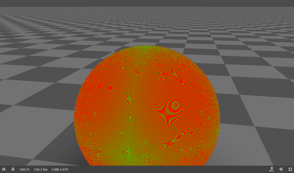
With all that, let’s quickly go over a few of the popular options; I have only considered a couple of popular options that target world space normals, of which there aren’t that many. In my experience, aside from being inconvenient to work with, view space normals tend to suffer from jittering artifacts since the values change every frame, whereas world normals are stable under movement even if quantization looks bad. I made a simple Shadertoy for visual comparison, and a bit of C++ code to compute the actual error values by iterating through all points on the sphere. All options are packed in 24 bits. For implementation ease I used my own HLSL++ library. I have computed the error metric as a difference between the two points on the sphere instead of an angular metric as the precision of acos() created many artifacts in vectors with very small differences. It should be close anyway for a unit sphere. Íñigo Quílez made a much more comprehensive comparison.

Trivial Encoding

1 2 3 4 float3 PackNormalTrivial(float normal) {     return normal * 0.5 + 0.5; }	1 2 3 4 float3 UnpackNormalTrivial(float3 packed) {     return packed * 2.0 - 1.0; }
1 2 3 4 5 v_add_f32     v1, v2, -0.5 mul:2 v_add_f32     v2, v3, -0.5 mul:2 v_add_f32     v0, v0, -0.5 mul:2   Total Instructions: 3	1 2 3 4 5 v_add_f32     v1, v2, 1.0 div:2 v_add_f32     v2, v3, 1.0 div:2 v_add_f32     v0, v0, 1.0 div:2   Total Instructions: 3

This is the baseline. It’s the cheapest, but its quality at 24 bits is inadequate to properly represent normals. Its average error is an order of magnitude worse than any of the options below. The main reason for this is that this encoding is able to represent a lot of redundant data, directions that are essentially the same after normalization but still require bits to represent.

CryEngine 3 Stereographic

1 2 3 4 5 6 float2 PackNormalStereographic(float3 normal) { float2 packed = normal.xy / (1.0f - normal.z); packed = packed * 0.5f + 0.5f; return packed; }

1 2 3 4 5 6 7 8 9 10 float3 UnpackNormalStereographic(float2 packed) { float2 unpacked = packed * 2.0f - 1.0f; float dotUnpacked = dot(unpacked, unpacked); float denominator = 1.0f + dotUnpacked; float3 result; result.xy = 2.0f * unpacked.xy / denominator; result.z = (-1.0f + dotUnpacked) / denominator; return normalize(result); }

1 2 3 4 5 6 v_sub_f32     v2, 1.0, v2 v_rcp_f32     v2, v2 v_fma_f32     v1, v3, v2, 1.0 div:2 v_fma_f32     v0, v0, v2, 1.0 div:2   Total Instructions: 4

1 2 3 4 5 6 7 8 9 10 11 12 13 14 15 16 17 18 19 v_add_f32     v3, v2, -0.5 mul:2 v_add_f32     v1, v0, -0.5 mul:2 v_fma_f32     v2, v3, v3, 1.0 v_fmac_f32    v2, v1, v1 v_rcp_f32     v2, v2 v_mul_f32     v0, v3, v2 mul:2 v_fma_f32     v3, v3, v3, -1.0 v_mul_f32     v4, v1, v2 mul:2 v_fmac_f32    v3, v1, v1 v_mul_legacy_f32  v1, v0, v0 v_mul_f32     v3, v3, v2 v_fmac_f32    v1, v4, v4 v_fmac_f32    v1, v3, v3 v_rsq_f32     v2, v1 v_mul_legacy_f32  v0, v0, v2 v_mul_legacy_f32  v1, v4, v2 v_mul_legacy_f32  v2, v3, v2   Total Instructions: 17

The stereographic encoding is a classic derived from the Stereographic Projection used for maps. It looks promising in terms of cost and error metrics, but (and the image already hints at it) we can see how the error distribution clearly favors one direction over another. At 24 bits this might be acceptable but lowering the bitrate will cause some normals to degrade much faster than others. This type of characteristic was exploited for view space normals, but Crytek seems to have been able to use that for world space normals.

Octahedral

1 2 3 4 5 6 7 8 9 10 float2 PackNormalOctahedral(float3 normal) { normal /= (abs(normal.x) + abs(normal.y) + abs(normal.z)); normal.xy =           normal.z >= 0.0 ?           normal.xy :           (1.0 - abs(normal.yx)) * select(normal.xy >= 0.0, 1.0, -1.0); normal.xy = normal.xy * 0.5 + 0.5; return normal.xy; }

1 2 3 4 5 6 7 8 9 10 float3 UnpackNormalOctahedral(float2 packed) { packed = packed * 2.0 - 1.0; // https://twitter.com/Stubbesaurus/status/937994790553227264 float3 n = float3(packed.xy, 1.0 - abs(packed.x) - abs(packed.y)); float t = saturate(-n.z); n.xy += select(n.xy >= 0.0, -t, t); return normalize(n); }

1 2 3 4 5 6 7 8 9 10 11 12 13 14 15 16 17 18 19 v_add_f32     v1, abs(v2), abs(v3) v_add_f32     v1, v1, abs(v0) v_rcp_f32     v1, v1 v_mul_f32     v4, v2, v1 v_mul_f32     v5, v3, v1 v_mul_f32     v0, v0, v1 v_cmp_ge_f32  s[0:1], v4, 0 v_fma_f32     v3, -abs(v3), abs(v1), 1.0 v_cmp_nle_f32  vcc, 0, v0 v_fma_f32     v0, -abs(v2), abs(v1), 1.0 v_cndmask_b32  v1, -v3, v3, s[0:1] v_cmp_ge_f32  s[0:1], v5, 0 v_cndmask_b32  v1, v4, v1, vcc v_add_f32     v1, v1, 1.0 div:2 v_cndmask_b32  v0, -v0, v0, s[0:1] v_cndmask_b32  v0, v5, v0, vcc v_add_f32     v0, v0, 1.0 div:2   Total Instructions: 17

1 2 3 4 5 6 7 8 9 10 11 12 13 14 15 16 17 18 19 20 21 v_add_f32     v1, v2, -0.5 mul:2 v_add_f32     v0, v0, -0.5 mul:2 v_add_f32     v2, -abs(v1), 1.0 v_cmp_le_f32  vcc, 0, v1 v_cndmask_b32  v5, 0, lit(0x80000000), vcc v_add_f32     v4, v2, -abs(v0) v_cmp_le_f32  vcc, 0, v0 v_cndmask_b32  v3, 0, lit(0x80000000), vcc v_med3_f32    v2, -v4, 0, 1.0 v_xor_b32     v5, v2, v5 v_xor_b32     v2, v2, v3 v_add_f32     v3, v1, v5 v_add_f32     v1, v0, v2 v_mul_legacy_f32  v2, v3, v3 v_fmac_f32    v2, v1, v1 v_fmac_f32    v2, v4, v4 v_rsq_f32     v2, v2 v_mul_legacy_f32  v3, v3, v2 v_mul_legacy_f32  v0, v1, v2   Total Instructions: 19

Octahedral is the most popular way of encoding to encode world space normals in the graphics world as far as I’m aware. The error distribution is more uniform so it can be used with lower bitrates and the ALU cost is competitive. Conceptually, we are trying to map the set of normals to the octants of an octahedron. This octahedron is mapped to the 2D plane and reconstructing the normal is a matter of knowing which octant the normal lies in.

Since we devote all bits to the points on the surface of the octahedron, we cannot really represent any vector inside or outside of it, which means all our bits are devoted to unique directions. The error distribution around the octants is apparent by looking at the image.

Epilogue

We clearly touched on a lot of topics here but I wanted to give a holistic and ordered approach to all the different ways I know of to pack data; from cramming colors into as few bits as possible, representing data in the arcane floating formats and encoding normals via octahedral magic, these techniques save memory and bandwidth to make your processor happy. Hopefully you can apply these building blocks to the many different domains within programming where it makes sense and have fun optimizing your data. I would like to thank @vassilis3d, @moguzhan_k and @aortizelguero for helping me out with readthroughs, feedback and good humor.